

Basic Survey Computations
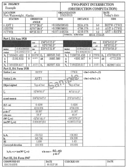
This appendix contains recommended procedures for performing basic survey computations. Until recently, three different forms were used to compute a two-point intersection. Army units have developed a one-sheet format (Figure C-1) to use when computing a two-point intersection. This one-sheet format is broken down into three parts and combines portions of DA Forms 1920, 1938, and 1947. Part I is from DA Form 1920, Part II is from DA Form 1938, and Part III is from DA Form 1947.
|
COMPUTATION OF A TWO-POINT IINTERSECTION
C-1. Tabulate data (known and field) for a two-point intersection on DA Form 1962 (Figure C-2) or on a blank piece of paper with an identifying heading. Include the following information:
- A properly oriented sketch of the triangle with the known baseline stations, an unknown station, and any other information that may be needed to organize computations. Label the unknown point as number 1 and the known points (clockwise from the unknown point) as number 2 and number 3.
- The position and elevation of known stations.
- The grid azimuth and grid distance of the known baseline.
- The observed horizontal angles, ZDs, and HIs.

|
NOTE: The grid azimuth (denoted by t) and the grid distance may be computed on DA Form 1934 by using UTM coordinates. If needed, conversions can be computed on DA Forms 1932 and 1933.
COMPLETE PART I OF THE ONE-SHEET FORMAT
C-2. Perform the following steps to complete Part I (Figure C-1) :
Step 1. Abstract all pertinent information from DA Form 1962 onto Part I. Include the following information:
- Record the—
- Record the station names (under the station column) opposite their respective numbers. Station 1 (unknown station) and Stations 2 and 3 (known stations).
- Record the observed horizontal angles opposite their respective numbers under the observed-angle column.
- Record the distance of the given side (side 2-3) that serves as the baseline under the distance column.
- Record the station names that correspond to each side under the side column.
Step 2. Complete the following items in Part I:
- Compute the unknown angle (number 1) by subtracting the two observed angles from 180°.
- Compute the sine of angle number 1 and record to nine decimal places with the sign (round the answer).
- Compute the side/sine ratio (denoted by D) by dividing the distance of the given side (side 2-3) by the sine of angle number 1 and record to six decimal places (round the answer).
- Compute the sine of angle number 2 and record to nine decimal places with the sign (round the answer).
- Compute side 1-3 by multiplying the sine of angle number 2 by D and record to three decimal places (round the answer).
- Compute the sine of angle number 3 and record to nine decimal places with the sign (round the answer).
- Compute side 1-2 by multiplying the sine of angle number 3 by D and record to three decimal places (round the answer).
COMPLETE PART II OF THE ONE-SHEET FORMAT
C-3. Perform the following steps to complete Part II (Figure C-1):
Step 1. Abstract all necessary information from DA Forms 1962 and Part I onto Part II. Record the—
- Project name.
- Project location.
- Organization performing the survey.
- Ellipsoid name.
- Zone number.
- Meridian designation.
- t (2 to 3).
- t (3 to 2).
- Angle at Station 2 (Ð 2).
- Angle at Station 3 (Ð 3).
- Northing and easting of Station 2 (N2 and E2).
- Northing and easting of Station 3 (N3 and E3).
- Station names opposite their appropriate numbers (for example, 2 ABE, 1 Pole, or 3 CAT).
- Grid distance of side 1-2 (from Part I).
- Grid distance of side 1-3 (from Part I).
Step 2. Complete the following items:
- Compute t (2 to 1) by adding Ð 2 to t (2 to 3). If the sum exceeds 360°, subtract 360°.
- Compute the sine of t (2 to 1). Record to nine decimal places with the sign (round the answer).
- Compute the dE by multiplying the sine of t (2 to 1) by the grid distance of side 2-1. Record to three decimal places with the sign (round the answer).
- Compute E1 by algebraically adding dE and E2. Record to three decimal places.
- Compute the cosine of t (2 to 1). Record to nine decimal places with the sign (round the answer).
- Compute the dN by multiplying the cosine of t (2 to 1) by the grid distance of side 2-1. Record to three decimal places with the sign (round the answer).
- Compute N1 by algebraically adding dN and N2. Record to three decimal places.
- Compute t (3 to 1) by subtracting the Ð 3 from t (3 to 2). If Ð 3 is larger than t (3 to 2), add 360° before subtracting.
- Compute the sine of t (3 to 1). Record to nine decimal places with the sign (round the answer).
- Compute dE by multiplying the sine of t (3 to 1) by the grid distance of side 3-1. Record to three decimal places with the sign (round the answer).
- Compute E1 by algebraically adding dE and E3. Record to three decimal places.
- Compute the cosine of t (3 to 1). Record to nine decimal places with the sign (round the answer).
- Compute dN by multiplying the cosine of t (3 to 1) by the grid distance of side 3-1. Record to three decimal places with the sign (round the answer).
- Compute N1 by algebraically adding dN and N3. Record to three decimal places.
NOTE: Compare the two sets of N 1 and E 1 . They must agree to within 0.001. If they do not, then a math or abstraction error was made, and Part II must be recomputed.
COMPLETE PART III OF THE ONE-SHEET FORMAT
C-4. Perform the following steps to complete Part III (Figure C-1):
Step 1. Abstract all information from DA Forms 1962 and Part II onto Part III. Record the—
- Project name.
- Project location.
- Organization performing the survey.
- Date of computation.
- Name of the station whose elevation is known (Station 1, occupied).
- Name of the station whose elevation is unknown (Station 2, observed).
- Object sighted (for example, target or obstruction light).
- Mean observed ZD (denoted by ζ1).
- Mean latitude (denoted by f ) and the azimuth of a line (denoted by α ).
NOTE: The azimuth of a line is recorded to the nearest minute and is obtained from Part II. The mean latitude is obtained by converting the northings and eastings computed on Part II to geographic positions and then taking the mean of the latitudes.
- Weighted mean coefficient of refraction (0.5 - m). When this is not observed, use 0.4290.
- Grid distance (denoted by s) (from Part II).
- Elevation of the occupied station (denoted by h1) (from DA Form 1962).
- HI of the station occupied (from DA Form 1962).
Step 2. Compute the elevation by using the following formulas:
- Compute rho (denoted by ρ) sine 1″. Record to three decimal places (round the answer). ρ is the mean radius of curvature in the plane of the distance and will be given (it can be found on DA Form 1962).
![]()
where—
R = radius of curvature in the plane of the meridian (obtained from NIMA's table generating software)
N = radius of curvature in the plane of the prime vertical (obtained from NIMA's table generating software)
- Compute the correction for the earth's curvature (denoted by κ) in seconds (denoted by secs). Record to one decimal place (round the answer).
m = mean coefficient of refraction
- Compute (90° - ζ1 + κ). Record to one decimal place (00.1″) with the sign (κ must be converted to minutes and seconds if it is over 60″).
- Compute the tangent of (90° - ζ1 + κ). Record to nine decimal places with the sign (round the answer).
-
Compute h2 - h1. Record to three decimal places with the sign (round the answer).
h2 - h1 = s · tan(90° - ζ1 + κ)
- Compute the corrected elevation by algebraically adding (h2 - h1), h1, and HI.
- Repeat Part III, steps 1 and 2, for observations taken from the other end of the baseline.
- Sign and date the form.
NOTE: Compute the DE between the two computed elevations. Use the following formula to determine the AE:
Use the shortest of the two distances to the unknown point. If the DE is larger than the AE, check for math and abstraction errors. If none are found, the intersection does not meet specifications and needs to be reobserved.
COMPUTATION OF A GRID TRAVERSE AND SIDE SHOTS
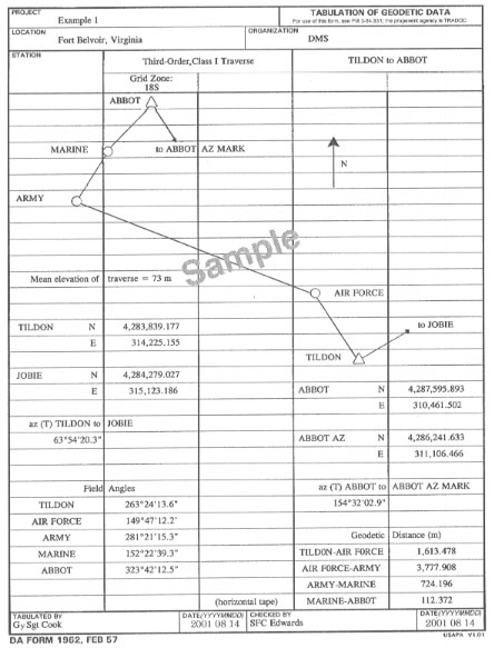
C-5. DA Form 1940 is used to compute a grid traverse. Tabulate known and field data for the traverse on a DA Form 1962 (Figure C-3) or on a blank piece of notepaper with an identifying heading. Include the following:
- A sketch of the traverse. Include the starting and ending stations, the intermediate stations, and any other information that may be needed to organize the computations.
- The position, the elevation, and the azimuth (if known) for the starting and ending stations.
- The observed angles and distances.
|
C-6. Figure C-4 shows a completed DA Form 1940. This figure is further broken down into separate figures to demonstrate the computation process. Refer to Figures C-5 and C-6 when working step 1 and Figure C-7 when working steps 2 through 7.
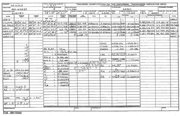
|
|

|
|
Step 1. Transfer the information from DA Form 1962 to DA Form 1940. Record the following information:
- Project name.
- Project location.
- Organization performing the survey.
- From station (starting station).
- To station (ending station).
- Number of angle stations (number of observed field angles).
- Grid zone.
- Traverse station names (the first and last columns of DA Form 1940).
- Observed angles (corrected mean station angles).
- Corrected field distances.
- Starting and ending projected geodetic azimuths (denoted by T).
- Mean elevation.
- Starting and ending UTM grid coordinates.
NOTE: The starting and ending T may be obtained from UTM coordinates by computing t and (t - T) on DA Form 1934.
Step 2. Compute the summation of angles (∑ Ðs) by adding all of the observed angles to the starting back azimuth. Leave the sum in decimal degrees. Record on DA Form 1940 to six decimal places (round the answer).
Step 3. Compute the ending azimuth by subtracting 180º from the ∑ Ðs until it is as close as possible to the known ending azimuth. Record on DA Form 1940 in degrees, minutes, and seconds. Record seconds to one decimal place (round the answers).
Step 4. Compute the AEC by subtracting the fixed (known) ending azimuth from the computed ending azimuth. Compute to one decimal place with the sign. Record in the "Total Angular Closure" block on DA Form 1940.
NOTE: The AEC is always equal to the computed values minus the fixed values as shown in the following formula:
Step 5. Compute the allowable AEC by using the formula from DMS Special Text (ST) 031. Since this is a third-order, Class I traverse, the formula used for computing the AE is ±10″![]() , where N is the number of segments or distances. This traverse has four distances; therefore AE = ±10″
, where N is the number of segments or distances. This traverse has four distances; therefore AE = ±10″![]() = ±20.0″.
= ±20.0″.
NOTE: The AE is always truncated. Do not round up the AE, because rounding will allow more error. Record to one decimal place.
Step 6. Compute the correction per station by dividing the AEC by the number of observed angles, then change the sign of the answer. Record to two decimal places with the sign, and truncate the answer.
NOTE: No one angle contains more of the error than another since the angular error is accidental. The error must be distributed evenly among the station angles.
Step 7. Compute the correction per observed angle and properly assign corrections to be applied to the observed angles. Record to one decimal place with the sign. After computing the correction per station, if the division does not result evenly to 0.1″, produce a group of corrections that are within 0.1″ of each other as in the following example.
C-7. After computing the correction per angle, assign the proper correction to each angle. For uniformity, apply the larger corrections to the larger angles. Record the correction per station in the "Angular Closure Per Station" block on DA Form 1940 (for example, 2 @ +2.0″ and 3 @ +1.9″). Sum the corrections. Record in the appropriate block on DA Form 1940.
NOTE: The sum of the corrections must equal the AEC, with the opposite sign. For example, if the AEC is negative, the corrections will be positive. If the AEC is positive, the corrections will be negative.
C-8. Refer to Figure C-8 for working steps 1 through 4.
|
Step 1. Compute the adjusted angles by algebraically adding the correction per angle to the observed angle. Record to one decimal place.
Step 2. Compute the azimuth of each traverse section by adding the first adjusted angle to the starting back azimuth. If the azimuth is over 360º, subtract 360º. This is the azimuth to the forward station. The azimuth of all lines must always be stated in the direction that the traverse is being computed.
Step 3. Convert the forward azimuth of the line to a back azimuth by either adding or subtracting 180º from the forward azimuth. The forward azimuth to the next station is then computed by adding the back azimuth from the previous line to the adjusted angle of the next station. If the new forward azimuth to the station is greater than 360º, subtract 360º.
Step 4. Repeat this procedure until the final station obtains a perfect check. The computed closing azimuth must agree exactly with the known closing azimuth. If not, a math error has been made and must be corrected.
NOTE: It is very important that particular attention be given to the direction of the azimuth. An error of 180º may go undetected, and two errors of 180º will cancel out (providing a final azimuth check). This will result in some sections being reversed in direction. Always refer to the sketch provided with the surveyor's field notes.
C-9. Refer to Figure C-9 when working steps 1 through 10.

|
Step 1. Compute the SLC. Record to six decimal places.
![]()
where—
h = the mean elevation
R = the mean radius of the earth (If h is in feet, use R = 20,906,000 feet. If h is in meters, use R = 6,372,000 meters.)
Step 2. Compute the middle northing (denoted by MID N) and the middle easting (denoted by MID E). To compute the MID N, add the northing of the beginning traverse station to the northing of the ending traverse station. Then divide by two. Record to the nearest 1,000 meters. To compute the MID E, add the easting of the beginning traverse station to the easting of the ending traverse station. Then divide by two. Record to the nearest 1,000 meters.
NOTE: A scale factor (denoted by K) is required to convert a measured distance to a grid distance. A mean K may be computed for the entire traverse or for each section in the traverse. For this example, a single K will be used since the traverse's total length is 8,000 meters or less. Traverses over 8,000 meters require a K to be computed for each section. Compute the northing and easting of the midpoint for the desired traverse or section to the nearest 1,000 meters. Record the formula in the appropriate block on DA Form 1940.
Step 3. Compute K. Record to six decimal places (round the answer).
K = Ko[1 + (XVIII)q2 + 0.00003 q4]
where—
Ko = the scale factor at the CM (0.9996)
XVIII = the Table 18 value
q = a factor used to convert E′ to millionths
Step 4. Obtain the Table 18 (denoted by XVIII) value. The XVIII value is extracted from the tables in DMS ST 045, using the MID N as the argument. Interpolate to compute the XVIII value to six decimal places (round the answer). An example follows:
Step 5. Compute E′ by subtracting 500,000 from the MID E. Record to 1,000 meters as an absolute value.
E′ = MID E - 500,000 = 312,000 - 500,000 = -188,000 m
where—
E′ = absolute value of MID E
Step 6. Compute q by multiplying E′ by 0.000001. Record to six decimal places (round the answer).
q = E′ · 0.000001 = 188,000 · 0.000001 = 0.188000
where—
q = a factor used to convert E′ millionths
Step 7. Compute q2 and q4. Record to six decimal places (round the answers).
q2 = 0.1880002 = 0.035344
q4 = 0.1880004 = 0.001249
Step 8. Compute K. Record to six decimal places (round the answer).
K = Ko[1 + (XVIII) q2 + 0.00003 q4]
= 0.9996[1 + 0.012318 · 0.035344 + 0.00003 · 0.001249]
= 1.000035
where—
Ko = the scale factor at the CM (0.9996)
q = a factor used to convert E′ millionths
Step 9. Compute a scale factor used to reduce the grid distance (denoted by k«) by multiplying K by the SLC. Record to six decimal places (round the answer).
K« = K · SLC = 1.000035 · 0.999989 = 1.000024
NOTE: After computing K and K«, record the values in the "Scale Factor x SLC" blocks on DA Form 1940 beside the appropriate corrected field distance.
Step 10. Compute grid distances as follows.
- Taped distances (corrected horizontal field distances) are reduced to grid distances by multiplying the taped distance by K«.
G = H · K«
where—
G = grid distance
H = taped distance
- EDME distances (reduced geodetic distances) are corrected by multiplying the geodetic distance by K.
G = S · K
where—
G = grid distance
S = geodetic distance
NOTE: Compute the total length of the traverse. Record to three decimal places in the "Length of Traverse" block on DA Form 1940 (Figure C-10).
|
C-10. Refer to Figure C-11 when working steps 1 through 3:
|
Step 1. Compute the cosines and sines of the azimuths. Record to seven decimal places with the sign (round the answer).
Step 2. Compute the dNs and the dEs.
- The dN is computed by multiplying the grid distance by the cosine of the azimuth. Record to three decimal places with the sign (round the answer).
dN = grid distance · cos (t)
- The dE is computed by multiplying the grid distance by the sine of the azimuth. Record to three decimal places with the sign (round the answer).
dE = grid distance · sin (t)
Step 3. Compute errors in the dN and the dE (denoted by En and Ee).
En = computed dN - fixed dN
Algebraically add the column of dNs to get the computed dN. Record to three decimal places with the sign.
Subtract the fixed starting northing from the fixed ending northing to get the fixed dN. Record to three decimal places with the sign.
En = computed dN - fixed dN = +3,756.391 - (+3,756.716) = -0.325
-
Compute the Ee by using the following formula. Record to three decimal places with the sign.
Ee = computed dE - fixed dE
Algebraically add the column of dEs to get the computed dE. Record to three decimal places with the sign.
Subtract the fixed starting easting from the fixed ending easting to get the fixed dE. Record to three decimal places with the sign.
Ee = computed dE - fixed dE = -3,763.327 - (-3,763.613) = +0.286
C-11. Refer to Figure C-12 when working steps 1 through 5.
Step 1. Compute the LEC. Record to four decimal places in the "Linear Closure Ratio" block on DA Form 1940. Compute the LEC by using the following formula:

|
Step 2. Compute the RC. Round down to the nearest 100. Record in the "Linear Closure Ratio" block on DA Form 1940. Compute the RC by dividing the length of traverse (in meters) by the LEC. Use the following formula:
Step 3. Compute the AE for position closure. Since this is a third-order, Class I traverse, the AE for position closure is equal to 0.4 times the square root of the distance of the traverse in kilometers. Compute the AE for position closure by using the following formula (found in DMS ST 031) (truncate and record the answer to four decimal places):
![]()
where—
k = the distance of the traverse in kilometers
NOTE: The LEC must be compared to the AE. If the LEC is equal to or less than the AE, the traverse has met specifications. If the LEC is greater than the AE, no further computations are necessary.
Step 4. Compute the correction factors (correction to northing [denoted by KN] and correction to easting [denoted by KE]) to be used in adjusting the traverse.
- KN is computed by dividing the En by the length of traverse in meters then changing the sign of the answer. Record to seven decimal places with the sign (round the answer).
- KE is computed by dividing the Ee by the length of traverse in meters then changing the sign of the answer. Record to seven decimal places with the sign (round the answer).
NOTE: A correction factor will always have the opposite sign of the En and the Ee.
Step 5. Compute corrections to dNs and dEs.
- Corrections to dNs are computed by multiplying KN by the grid distance. This is done for each section of the traverse. Record to three decimal places with the sign (round the answer).
- Corrections to dEs are computed by multiplying KE by the grid distance. This is done for each section of the traverse. Record to three decimal places with the sign (round the answer).
- After all the corrections are recorded, sum the columns. The sum of the corrections must equal the errors of dN and dE with the opposite sign. If, because of rounding errors, the sum does not exactly equal the error of dN or dE, this difference must be distributed. For uniformity, the largest corrections are changed by one unit (third decimal place) until the correct sum is obtained.
- The sum of the dN corrections is exactly equal to the error (-0.325) with the opposite sign.
- The sum of the dE corrections is different by 0.001 from the error (+0.286). Therefore, an additional 0.001 is applied to the largest correction (0.173).
C-12. Refer to Figure C-13 when working steps 1 and 2.
|
Step 1. Compute the adjusted grid coordinates (northings and eastings).
- To compute the adjusted northing, algebraically add the dN and the correction of dN to the northing of the preceding station. Record to three decimal places.
- To compute the adjusted easting, algebraically add the dE and the correction of dE to the easting of the preceding station. Record to three decimal places.
NOTE: Continue in a like manner for each station. As a math check, apply the last dN and the last correction of dN to the northing of the preceding station. The answer must equal the fixed northing of the closing station. The same is true for the easting.
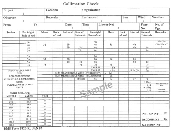
COMPUTATION OF A C-FACTOR
C-13. Compute the C-factor. Record on DMS Form 5820-R. Refer to Figure C-14 and Figure C-15 when working steps 1 through 15. The step numbers correspond to the numbered blocks on Figure C-14. Figure C-15 shows a completed DMS Form 5820-R.
Step 1. Complete the heading information (1).
Step 2. Record the stadia constant for the instrument (2).
Step 3. Record the backsight-rod (near-rod) readings (in millimeters) (3a).
- Compute and record stadia intervals (in millimeters) (3b). If the difference is greater than 3, reobserve.
- Compute and record the sum of the intervals (3c).
- Compute and record the mean middle-wire reading (in millimeters) to one decimal place (3d).
- Compute and record the sum of the three-wire readings (in millimeters) (3e).
Step 4. Record the foresight-rod (far-rod) readings (in millimeters) (4a).
- Compute and record the stadia intervals (in millimeters) (4b). If the difference is greater than 3, reobserve.
- Compute and record the sum of the intervals (4c).
- Compute and record the mean middle-wire reading (in millimeters) to one decimal place (4d).
- Compute and record the sum of the three-wire readings (in millimeters) (4e).
Step 5. Record the backsight-rod (near-rod) readings (in millimeters) (5a).
- Compute and record the stadia intervals (in millimeters) (5b). If the difference is greater than 3, reobserve.
- Compute and record the sum of the intervals (5c).
- Compute and record the mean middle-wire reading (in millimeters) to one decimal place (5d).
Step 6. Record the foresight-rod (far-rod) readings (in millimeters) (6a).
- Compute and record the stadia intervals (in millimeters) (6b). If the difference is greater than 3, reobserve.
- Compute and record the sum of the intervals (6c).
- Compute and record the mean middle-wire reading (in millimeters) to one decimal place (6d).
Step 7. Compute and record the cumulative totals as follows:
Step 8. Apply the correction for C&R. Due to the short distance from the instrument to the near rod, no corrections are required to the near-rod readings.
- Use the far-rod distance (4c ÷ 10) as an argument to determine the second correction. Table C-1 shows correction factors for C&R according to the observed distance. Record the correction from Table C-1 in the C&R number 1 block (8b).
- Use the far-rod distance (6c ÷ 10) as an argument to determine the correction. Record the correction from Table C-1 in the C&R number 2 block (8c).
- Correct the sum of the far-rod mean middle-wire readings for C&R. Algebraically add the sum of 8b and 8c to 7e. Since the correction is always negative, just subtract 8b and 8c from 7e (8d).
- Algebraically add 8d and 7b. Record the sum with the sign (8e). 8d is always negative.
Step 9. Compute the C-value by dividing 8e by 7g. Truncate and record to four decimal places with the sign (9).
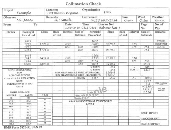
NOTE: If the sum of the far-rod mean middle-wire readings (8d) is larger than the sum of the near-rod mean middle-wire readings (7b), the C-value is negative.
Step 10. Compare the C-value with that allowed for the instrument. The allowable C-value in most instruments is +0.004. If the C-value is within specifications, no further computations are required.
Step 11. Correct the C-value if it is not within the specifications.
- The correction to the middle wire (in millimeters) is computed by multiplying the sum of the rod intervals of the last foresight (shown in 6c) by the C-value (shown in 9). Compute to one decimal place (round the answer) (11a).
- The correction to the middle wire (11a) is added algebraically to the last foresight middle-wire rod reading (shown in 6a) to obtain the corrected rod reading. Compute to three decimal places (divide the correction by 1,000 to convert to meters before applying) (round the answer) (11b).
Step 12. Initial the form (12).
Step 13. Perform field adjustments.
Step 14. Repeat steps 1 through 13 until the C-value is within specifications.
Step 15. Give the recording form to the instrument operator once it has been determined that the instrument is within specifications. The instrument operator will check the form for completeness and the computations for correctness and initial the form (15).
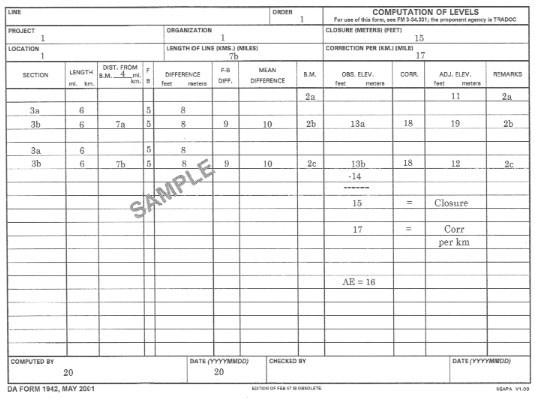
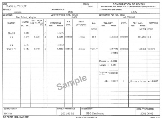
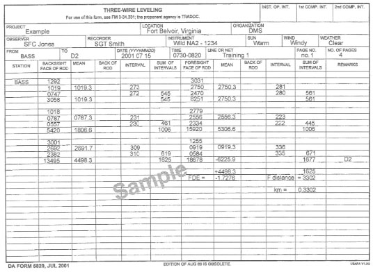
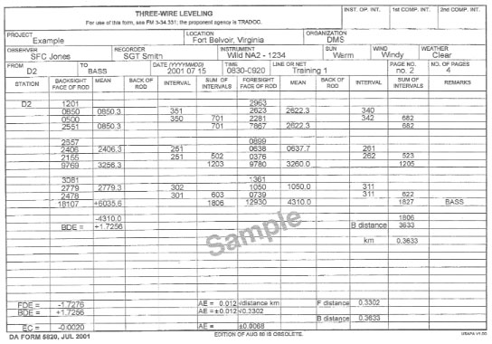
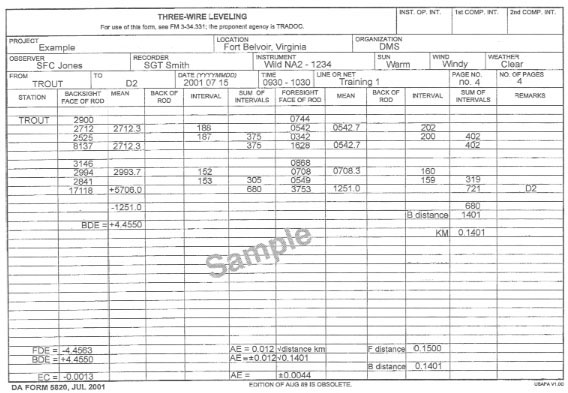
COMPUTATION OF A LEVEL LINE
C-14. Compute a level line on DA Form 1942. Refer to Figure C-16, when working steps 1 through 20 (the step numbers correspond to the numbered blocks). Figure C-17, shows a completed DA Form 1942. Data will be required from the field notes (DA Form 5820) shown in Figures C-18, C-19, C-20, and C-21.
Step 1. Complete the headings (1).
Step 2. Record the name of the—
Step 3. Record the name of the—
Step 4. Record the name of the beginning BM (4).
Step 5. Record the direction of the run (forward [F] or backward [B]) (5).
Step 6. Abstract the length of the forward and backward runs per section from the level field notes. Record to the nearest 0.001 kilometer, in their respective directions (6).
Step 7. Compute the length of the line by adding the shortest distance of each section of the level line (7a). Record the total length of the line (7b).
Step 8. Compute the observed DE of the forward and backward runs per section from the level field notes. Record to four decimal places with the sign (in their respective running directions) (8).
Step 9. Compute the DE between the forward and the backward runs per section. Record to four decimal places as an absolute value (no algebraic signs) (9).
Step 10. Determine the mean DE by computing the absolute mean of the forward and the backward DE. Give the mean DE the algebraic sign of the forward run. Record to four decimal places (round the answer) (10).
Step 11. Record the known elevation of the beginning BM (11).
Step 12. Record the known elevation of the ending BM (12).
Step 13. Compute the observed elevation by algebraically adding the mean difference (shown in 10) and the elevation of the beginning BM (shown in 11). Record to four decimal places (13a). Compute each successive observed elevation by algebraically adding it to the preceding elevation and the respective section's mean DE. Record to four decimal places (13b).
NOTE: The last entry will be the observed elevation of the ending BM. This entry must be compared to the fixed ending elevation.
Step 14. Record the known elevation of the ending BM (from step 12) (14).
Step 15. Compute the closure by subtracting the known elevation of the ending BM (shown in 14) from the computed observed elevation of the ending BM (shown in 13b). Record to four decimal places with the sign (15).
Step 16. Compute the AE. Truncate and record to four decimal places (16). For third-order specifications, use the following formula:
Km = length of line in kilometers (from 7b)
Compare the AE (16) to the closure (shown in 15). If the numerical value of the closure is equal to or smaller than the AE, the level line meets third-order specifications. If it does not, there is no need to continue with the computations on DA Form 1942.
Step 17. Compute the correction per kilometer. Divide the closure (shown in 15) by the total length of the line (shown in 7b) and change the sign. Record to six decimal places with the sign (round the answer) (17).
Step 18. Compute the correction for each section. Multiply the length of the line (shown in 7a) of each section by the correction per kilometer (shown in 17). Record to four decimal places with the sign (round the answer) (18).
NOTE: The correction to the final section must be equal to the closure (15), with the opposite sign.
Step 19. Compute the adjusted elevation. Algebraically add the correction (shown in 18) to the observed elevation (shown in 13a) of each station. Record to four decimal places (round the answer) (19).
Step 20. Sign and date the form (20).
|
|
|
|

|
|
|
NEWSLETTER
|
| Join the GlobalSecurity.org mailing list |
|
|
|