


D.2.0 METHODOLOGY
Risk associated with TWRS baseline and post-remediation conditions would result from long-term exposure to contaminants. Exposure would be controlled largely by how the land is used, and thus exposure scenarios based on land use serve as the basis for estimating risk. The five exposure scenarios selected for the analysis are the Native American, residential farmer, industrial worker, recreational shoreline user, and recreational land user. The Native American scenario was developed from the Columbia River Comprehensive Impact Assessment (Napier et al. 1996), which was modified at the request of and in consultation with the potentially affected Tribes. This scenario is in its initial stages of development and has not received a complete review by the scientific community, nor has it been approved by the potentially affected Tribes. Therefore, this scenario should be considered preliminary and may have more uncertainty associated with it than the other scenarios. However, the scenario does provide a bounding assessment of the potential health effects to a Native American who might engage in both subsistence lifestyle activities (e.g., hunting, fishing, and use of a sweat lodge) and contemporary lifestyle activities (e.g., irrigated farming). The residential farmer, industrial worker, recreational shoreline user, and recreational land user scenarios are modeled after scenarios in the Hanford Site Risk Assessment Methodology (HSRAM) (DOE 1995c). HSRAM was developed by an interagency working group for risk assessment that included technical representatives from the U.S. Department of Energy (DOE), the Washington State Department of Ecology (Ecology), and the U.S. Environmental Protection Agency (EPA). For each of the five scenarios analyzed, exposure to contaminants transported in four media is considered (i.e., groundwater, soil, surface water, and air).
By contrast, risk associated with operations for the TWRS remedial action alternatives would result from a shorter duration of exposure to contaminants. Such exposure would be largely controlled by the activities and processes associated with a particular remedial alternative or subalternative. The receptors for remediation risk are the TWRS workers, the noninvolved workers at the Hanford Site, and the public. Based on the assumptions listed in Table D.1.0.1, routine operations for the remedial action alternatives would result in atmospheric emissions of contaminants and potential direct radiation exposure from the waste. Air is the only transport medium considered.
Detailed descriptions of the methodology used are presented in Section D.2.1 for baseline and post-remediation risk and in Section D.2.2 for remedial action risk.
D.2.1 BASELINE AND POST-REMEDIATION RISK METHODOLOGY
A modular risk assessment (MRA) methodology was developed to analyze the risk associated with baseline and post-remediation conditions. The modular approach is based on separating the four basic components of the risk assessment process (i.e., source, transport, exposure, and risk) into discrete modules that can be assessed independently and then combined. The key concepts of the modular approach include the following:
- Defining the Hanford Site as a grid of cells, each 1 kilometer (km) by 1 km (0.6 mile [mi] by 0.6 mi);
- Aggregating contaminant sources located within each cell or several cells;
- Using transported unit concentrations (i.e., concentrations based on transport of a unit concentration of each contaminant) to develop concentration estimates at various locations as source terms vary;
- Using well-defined, land-use-based exposure scenarios;
- Using unit risk factors (URFs) (i.e., risk based on exposure to a unit concentration of each contaminant) to facilitate risk estimates as source terms vary; and
- Presenting risk in graphical contour plots developed using Geographic Information System (GIS) software.
The following is an overview of the modular risk-assessment approach.
The Hanford Site was divided into small sections or cells by superimposing a grid, based on state plane coordinates (Cartesian), on a map of the Hanford Site. All source cells (i.e., cells containing tank waste and other contaminant sources from TWRS EIS alternatives) were identified and the contaminants in the individual sources were quantified for both baseline and post-remediation conditions. Data for the individual sources were then aggregated for each source cell.
As an independent step, the release and transport of a unit of concentration of each contaminant from each source cell through different media was modeled for selected time periods ranging from the present to 10,000 years into the future. This time period was chosen because it is consistent with rationale presented by EPA in 40 Code of Federal Regulations (CFR) 191 for assessment of performance of repositories for disposal of radioactive waste. Modeling predicts how a unit concentration of each contaminant moves through the environment into surrounding cells after release from the source cell. This step results in transported unit concentrations for each medium and time period of interest.
Also as an independent step, a URF was calculated based on the dose to a receptor from exposure to a unit of concentration of each contaminant under each land-use scenario. Each scenario was evaluated for all potential transport media. The resultant risk values then were calculated. The source (baseline or post-remediation) was multiplied by the transported unit concentration at the selected time to obtain the future concentration of the source in a given cell (referred to as point concentration). The point concentration then was multiplied by the URF for the given land-use scenario to obtain the risk to a receptor in that cell. This process can be described in the following general equation:
(Risk Value) = (Source) · (Unit Transport Factor) (URF)
In the MRA methodology, four data sets were developed for each cell. These data sets consist of the individual source data, transported unit concentrations, URFs, and risk values, which are calculated by multiplying the values in the other three data sets for a given land use. Each of these data sets was considered a module. A computerized spreadsheet was developed for each module to facilitate storage and mathematical manipulation of the data.
In converting exposures to risk, the primary source for health effects conversion factors is the International Commission on Radiological Protection (ICRP) Publication No. 60 (ICRP 1991), which recommends values for the public of 5.0E-04 fatal cancers per rem and 1.0E-04 nonfatal cancers per rem, for a total cancer incidence of 6.0E-04 per rem. The cancer incidence calculations for chemicals and radionuclides based on EPA slope factors include fatal plus nonfatal cancers. The EPA slope factors are not based on use of a single health effects conversion factor, but consider age-specific and organ-specific health risk in estimating the slope factors. EPA suggested use of 7.3E-04 total cancers per rem (for member of the public) for those radionuclides for which slope factors are not provided (by EPA). This factor is not used for analysis.
The modules developed for this risk assessment (i.e., source, unit transport, URF, and risk) are described in more detail in the following sections. The source module is described in Section D.2.1.1 followed by the unit transport module (Section D.2.1.2) and URF module (Section D.2.1.3). The combination of these factors give s an estimate of the human health impacts as described in Section D.2.1.4.
D.2.1.1 Source Module
The source module contains information identifying and quantifying the sources of contamination under current and post-remediation conditions. To assess risk from exposure to contaminants transported through the environment, the amount of the contaminant that would be released into the environment was determined. The amounts released, referred to as release terms, are a calculated fraction of the total contaminant inventories available for release. Release terms are developed as part of the transport modeling process and are discussed in Section D.2.1.2. Contaminant inventories available for release comprise the data tabulated in the source module and are discussed in this section. These inventories are contaminant-specific and given as either inventory amounts or concentrations.
The source module for this assessment is divided into submodules, as shown in Table D.2.1.1. For each submodule shown, contaminant inventories are compiled and tabulated for use in the risk calculation.
Table D.2.1.1 Elements of the Source Module
For post-remediation conditions, source inventories are tabulated for the contamination sources estimated to exist after remedial actions are completed. Depending on the alternative, the anticipated post-remediation sources would consist of tank residuals, in situ disposed tank waste, and engineered storage/disposal facilities. The inventories for these sources are based on engineering analyses of the remedial action alternatives provided in a set of engineering data packages prepared to support this EIS (WHC 1995c, 1995d, 1995e, 1995f, 1995g, 1995h, 1995i, 1995j, and 1995n, and Jacobs 1996). Additional discussion of current and post-remediation inventories is presented in the following sections.
D.2.1.1.1 Current Tank Waste Inventories
Current tank waste inventories were obtained from a supporting document for this EIS (WHC 1995d). Tank inventories are displayed on a total tank basis only (i.e., total inventory for single-shell tanks [SSTs] and total inventory for double-shell tanks [DSTs]). Total-tank inventories are shown in Appendix A, Tables A.2.1.2 and A.2.1.3 for radionuclides and nonradioactive chemicals, respectively.
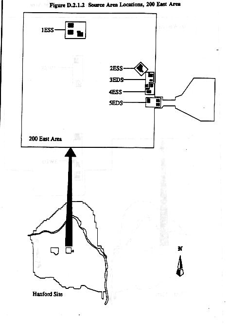
The groundwater transport modeling separated contaminant sources in the 177 tanks into eight aggregated source areas, each of which contained groupings of either SST farms or DST farms. Tank farms in the 200 West Area were grouped into three source areas, designated 1WSS, 2WSS, and 3WDS (Figure D.2.1.1). Tank farms in the 200 East Area were grouped into five source areas, designated 1ESS, 2ESS, 3EDS, 4ESS, and 5EDS (Figure D.2.1.2). The groupings were based on tank farm location, tank type (SST or DST), and groundwater flow direction.
Figure D.2.1.1 Source Area Locations, 200 West Area
Figure D.2.1.2 Source Area Locations, 200 East Area
To generate inventories for the eight source areas, computer spreadsheets were developed from the data used to generate the tables from (WHC 1995d and Jacobs 1996). The spreadsheets contained farm-by-farm inventories for SSTs and tank-by-tank inventories for DSTs, from which inventories were allocated among the eight source areas.
Quantities of radionuclides are dependent on the time period of interest because of the spontaneous decay of radionuclides. The quantities of radionuclides were available for SSTs for a range of dates, including the year 1995. However, the concentration of radionuclides for DSTs was available only for the year 1999. Because the year 1995 is the designated starting time (T0) for this risk assessment, a calculation was used to convert the DST inventory quantities to a December 31, 1995 date.
The calculation was performed using the following equation:
I(1999) = I(1995) e-
 t
t
Where:
I(1995) = Inventory year 1995
I(1999) = Inventory year 1999
= Decay constant = ln2/T1/2
t = Decay duration (1999 - 1995 = 4 years)
T1/2 = Radionuclide half-life
The short-lived progeny radionuclides were assumed to be in equilibrium with the parents.
Single-Shell Tanks
Current inventories for the five source areas containing SSTs are shown in Volume Two, Appendix A, Tables A.2.1.5 and A.2.1.6. Table A.2.1.5 shows the aggregated inventory of nonradioactive chemicals. Table A.2.1.6 shows the aggregated inventory of radionuclides for December 31, 1995 (totals for December 31, 1999 are also included for comparison purposes). The aggregated inventories were generated by summing the farm-by-farm inventories for the SST farms in each source area.
Double-Shell Tanks
Current inventories for the three aggregated source areas containing DSTs are shown in Volume Two, Appendix A, Tables A.2.1.7 and A.2.1.8. Table A.2.1.7 shows the aggregated inventory of nonradioactive chemicals. Table A.2.1.8 shows the aggregated inventory of radionuclides for December 31, 1995. The inventories were generated by summing tank-by-tank inventories for the DST in each source area.
Miscellaneous Underground Storage Tanks
There are approximately 40 inactive and 20 active MUSTs associated with the tank farms. These MUSTs contain small quantities of mixed radioactive and chemical waste. They contain less than one-half of one percent of the total tank farm inventory. Additional information on the MUST inventory can be found in Volume Two, Appendix A.
D.2.1.1.2 Current Cesium and Strontium Capsule Inventories
Radioactive decay calculations for Cs/Sr capsules stored at the Waste Encapsulation and Storage Facility (WESF) in the 200 East Area of the Hanford Site result in the following quantities:
- Cs: 1,328 capsules, 53.2 million curies (MCi) total inventory; and
- Sr: 601 capsules, 23.1 MCi total inventory.
D.2.1.1.3 Post-Remediation Inventories
The contamination sources anticipated to exist after remediation vary according to each alternative. These sources were identified and quantified based on engineering data packages developed by the Site Management and Operations contractor and the TWRS EIS contractor (WHC 1995c, d, e, f, g, h, j, n, and Jacobs 1996). Depending on the alternative, the post-remediation sources would consist of tank residuals, in situ disposed tank waste, and engineered storage/disposal facilities. Contaminant inventories were developed from the engineering data packages, and entered into the source module for each of these post-remediation sources.
Tables displaying the post-remediation inventories by source for each alternative are presented in Volume Four, Appendix F, Groundwater Modeling.
D.2.1.2 Transport Module
Transport refers to the movement of contaminants in the environment from the source location to the receptor. The transport analysis redistributes the contaminants at locations within and outside the grid cell sources. Transport of contaminants was modeled within the Hanford Site boundary and within an 80-km (50-mi) radius of TWRS facilities.
Development of release terms (i.e., the portion of current or post-remediation inventories in the source module that are estimated to be released from the source) is conducted as part of the transport analyses. Further discussions of the method for developing release terms, along with tables displaying the release terms used for each source, are provided in Volume Four, Appendix F for groundwater releases and in Volume Five, Appendix G for air releases.
Developing transport parameters for contaminants of concern in soil, groundwater, surface water, and air also is conducted during the transport analyses. Transport parameters consist of the contaminant- and site-specific data required to model the atmospheric, groundwater, and surface water transport of contaminants within and outside the boundaries of the Hanford Site. Transport parameters and radionuclide decay estimates result in new media concentrations specific to the location and time period of interest. Transport parameters are discussed further in Volume Four, Appendix F for groundwater transport and in Volume Five, Appendix G for air transport.
Transport modeling for this assessment was conducted as a unit transport analysis. This analysis involved modeling the transport of a single unit of contaminant from TWRS sources through the environment (groundwater, soil, air, and surface water) at different times in the future. Any cells that contain contaminants at the present time are set as the location of a unit inventory or concentration. A unit of contaminant is transported from one medium to other media and from a location (cell) to other locations, as time progresses, using a transport code. The transported unit concentration for each medium at selected modeling time periods (i.e., 300, 500, 2,500, 5,000, and 10,000 years in the future) is estimated and tabulated in the transport module. Point concentrations, which are the future concentrations at a given receptor originating from a particular source, are obtained by multiplying the current and post-remediation inventories by the transported unit concentrations at selected time periods.
D.2.1.3 Exposure Module
Five exposure scenarios were used as the basis for the unit risk calculations: Native American, residential farmer, industrial worker, recreational shoreline user, and recreational land user (DOE 1995c). The Native American scenario represents potential use of the land for a subsistence Native American lifestyle as well as contemporary lifestyle activities such as irrigated agriculture. This scenario includes subsistence activities such as hunting, fishing, and gathering of plants and materials. The residential farmer scenario represents potential use of the land for residential and agricultural production. This scenario includes producing and consuming animal, vegetable, and fruit products. The industrial worker scenario involves mainly indoor activities that include consumption of groundwater , although outdoor activities (e.g., soil contact) also are included. The recreational shoreline user was assumed only to have access to the Hanford Reach of the Columbia River. The recreational land user was assumed to be a random Sitewide land user of the Hanford Site, excluding the Columbia River shoreline. The exposure scenarios were evaluated for five transport media, as appropriate: 1) soil defined per unit mass; 2) soil defined per unit area; 3) groundwater from wells; 4) surface water (including shoreline sediments); and 5) air. Soil was evaluated by mass to account for contaminants transported through the soil, and by area to account for contaminants deposited onto the soil from atmospheric transport.
The exposure module for human receptors is based on land-use patterns. For each grid cell, the exposure pathway and receptors associated with that cell were identified. This was done by activating or deactivating transport media within the cell. For example, by activating the residential farmer scenario, groundwater would be used to irrigate crops that are consumed directly by the surrounding population, and by milk- and meat-producing cattle that are consumed by the surrounding population. By activating the recreational land-user scenario, the groundwater medium would not be included because the recreational land user is assumed not to be a resident of the land and is assumed not to consume water from the aquifer.
The URF is the risk associated with exposure to one concentration unit (e.g., risk per pCi/g for radionuclides in soil, risk per mg/kg for chemicals in soil, risk per pCi/L for radionuclides in water) of a given contaminant for a human exposure scenario. The URFs were developed for each individual exposure pathway (i.e., ingestion, inhalation, and direct contact) for each scenario. Slope factors developed by EPA (Integrated Risk Information System [IRIS] 1995 and Health Effects Assessment Summary Tables [HEAST] 1995) were applied. The exposure module contains a set of URF tables for each exposure scenario and receptor. The URF values presented in the tables of this report were based on the summation of all relevant exposure pathways. For example, the residential groundwater URF values would include ingestion of drinking water, dermal contact while showering, incidental ingestion while showering, and inhalation of volatile emissions from domestic use.
The calculation of URFs is simplified by dividing the equations into two main terms, one containing parameters independent of contaminant properties (summary intake factors) and the other containing parameters dependent on contaminant properties (contaminant-specific parameters). The following sections describe methods used to calculate each of these types of parameters; Section D.2.1.3.1 - Summary Intake Factors and Section D.2.1.3.2 - Contaminant-Specific Parameters. The use of these terms to estimate the URFs then is described in Section D.2.1.3.3 - Unit Risk Factors.
D.2.1.3.1 Summary Intake Factors
Exposure scenarios are described in terms of receptors, exposure media or pathways, and summary intake factor (SIF) values.
- The receptor is the type of human exposed in terms of age, weight, and exposure duration and other factors. Five receptors were modeled: Native American, residential farmer, industrial worker, recreational shoreline user, and recreational land user. Except where noted, receptor parameters used in the analysis are consistent with those established in HSRAM (DOE 1995c).
- The exposure pathway is the medium (e.g., groundwater) and activity (e.g., drinking) that would result in an exposure.
- The SIF value is the amount of exposure to the receptor through the media of interest. The SIF values were derived for each of three toxicity types: NC - noncarcinogenic chemicals, CC - carcinogenic chemicals, and RA - radionuclides.
The SIF concept is presented in HSRAM (DOE 1995c). The concept of SIF values involves structuring the intake equations for each exposure pathway so that contaminant-independent parameters are separated from the contaminant-specific parameters and the initial media concentration. Each exposure pathway model then can be described as the product of three factors: 1) a media concentration, 2) an SIF independent of the specific contaminants, and 3) a factor composed of all contaminant-specific parameters. The equation is as follows:

Where:
Intake = Average daily intake of chemical contaminants (mg/kg day)
Exposure = Total intake or exposure received over the exposure duration (pCi or hour)
Ciym = Concentration of contaminant i, of type y, in medium m (mg or pCi per unit quantity of medium liter, kilogram, m3, or m2)
PFmix = Contaminant-specific factor for medium m, contaminant i, and exposure pathway x (Strenge-Chamberlain 1994) (units specific to analysis)
SIFsmyx = Summary intake factor for scenario s, medium m, contaminant type y, and exposure pathway x (units specific to analysis)
The SIF values were evaluated for each toxicity type (i.e., NC, CC, and RA). The appropriate SIF value was used for each contaminant for the exposure pathway of concern. The methodology for calculating SIF values is described by Strenge and Chamberlain (Strenge-Chamberlain 1994). The SIF values for the five exposure scenarios are described in more detail in the following sections. This is followed by a discussion of the contaminant-specific factors.
Following loss of institutional controls (assumed to be 100 years), the tank contents would be released to subsurface soils and be available for transport to groundwater from infiltration of rainwater and percolation through the soil column. Based on the existing depth of the tanks, the resulting soil contamination would be below the maximum depth of soil likely to be contacted by all potential receptors, with the exception of the intruder scenario. Consequently, the soil medium was not evaluated as a post-remediation transport mechanism for any of the alternatives because the soil contamination was not evaluated for any of the alternatives. Therefore, groundwater is the only post-remediation transport mechanism evaluated for all of the alternatives.
Native American Scenario
This scenario represents exposures received during a 70-year lifetime by a Native American who engages in both traditional lifestyle activities (e.g., hunting, fishing, and using a sweat lodge) and contemporary lifestyle activities (e.g., irrigated farming). The individual is assumed to spend 365 days per year on the Site over a 70-year lifetime. Some activities are assumed to continue year-round while others are limited by climate (e.g., frost-free days).
Pathways for this scenario include those defined for the residential farmer scenario in HSRAM, plus additional pathways representing activities unique to the Native American subsistence lifestyle (e.g., exposures in a sweat lodge). A composite adult was used as the receptor for some of the pathways. The composite adult was evaluated using child parameters for 6 years and adult parameters for 64 years. The child's body weight was assumed to be 16 kilograms (kg) (35 pounds [lbs]), and the adult body weight 70 kg (150 lbs). This approach was used for all contaminant types. Table D.2.1.2 presents the pathways included in the Native American scenario. The exposure parameters for each pathway are presented in Table D.2.1.3. The SIF values for each pathway are presented in Table D.2.1.4.
Table D.2.1.2 Exposure Pathways Included in Native American Scenario
Table D.2.1.3 Native American Scenario Exposure Factors
Table D.2.1.4 Native American Scenario Summary Intake Factors
The ingestion rates of native foods are based on a combination of EPA-suggested intake rates (EPA 1989b), intake rates used for the Columbia River Comprehensive Impact Assessment (Napier et al. 1996), and data provided by the affected Tribes. Ingestion of animal organs and wild bird meat was accounted for by increasing the total meat intake rate. Animal organs were assumed to have contaminant concentrations 10 times the concentration in other animal tissue, and the organ intake rate was assumed to be 10 percent of the intake rate of other animal tissue. Animal meat plus organ intake was assumed to be 300 g/day. Intake of upland game birds and waterfowl was assumed to be 9 g/day and 35 g/day, respectively. The total meat ingestion rate was thus assumed to be 341 g/day. Ingestion of fish organs was accounted for by increasing the fish muscle intake rate in a manner similar to that for ingestion of animal organs. Fish organs were assumed to have contaminant concentrations 10 times the concentration in fish muscle, and the fish organ ingestion rate was assumed to be 10 percent of the fish muscle intake. The total fish ingestion rate was assumed to be 1,080 g/day.
This scenario, by incorporating the subsistence lifestyle activities and native food ingestion rates as described above, results in exposures that are approximately five times higher than the exposures for the residential farmer scenario.
Residential Farmer (Agricultural) Scenario
This scenario represents use of the land for residential and agricultural production. This scenario includes producing and consuming animal, vegetable, and fruit products. The exposures are assumed to be continuous and include occasional surface water-related recreational activities, which include contact with surface water sediments. A composite adult was used as the receptor for some of the exposure pathways. The composite adult was evaluated using child parameters for 6 years and adult parameters for 24 years, with a total exposure duration of 30 years. The child's body weight was assumed to be 16 kg (35 lbs), and the adult body weight 70 kg (150 lbs). This approach was used for all contaminant types. Table D.2.1. 5 presents the pathways included in the residential farmer scenario. The exposure parameters for each pathway are presented in Table D.2.1. 6 . The SIF values for each pathway are presented in Table D.2.1.7 .
Table D.2.1.5 Exposure Pathways Included in Residential Farmer Scenario
Table D.2.1.6 Residential Farmer Scenario Exposure Factors
Table D.2.1.7 Residential Farmer Scenario Summary Intake Factors
The ingestion rates of farm products for the residential farmer are based on EPA-suggested intake rates (EPA 1989b). The individual was assumed to consume a total of 200 g/day of vegetables of which 40 percent is homegrown and contaminated; 140 g/day of fruit of which 30 percent is homegrown and contaminated; 100 g/day of beef of which 75 percent is contaminated; and 300 g/day of dairy products of which 75 percent is contaminated. These intake rates are used by HSRAM and described by EPA as representing reasonable bounding estimates.
Industrial Scenario
The industrial scenario represents potential exposures to workers in a commercial or industrial setting. The receptors are adult employees assumed to work at this location for 20 years and have an average body weight of 70 kg (150 lbs).
The scenario involves mainly indoor activities, although outdoor activities (e.g., soil contact) also are included. These exposures would not be continuous because the worker would go home at the end of each work day. The scenario is intended to represent nonremediation workers assumed to wear no protective clothing. Table D.2.1. 8 presents the pathways included in this scenario. The exposure parameters for each pathway are presented in Table D.2.1. 9 . The SIF values for each pathway are presented in Table D.2.1. 10 .
Table D.2.1.8 Exposure Pathways Included in Industrial Scenario
Table D.2.1.9 Industrial Scenario Exposure Factors
Table D.2.1.10 Industrial Scenario Summary Intake Factors
Recreational Shoreline User Scenario
The recreational shoreline user scenario represents exposure to contamination in the Columbia River and shoreline from recreational swimming, boating, and other shoreline activities. The scenario involves outdoor activities. These exposures would not be continuous, but would occur for 14 days/year for 30 years. Exposures to both adults and children were taken into account using the composite adult described for the residential farmer scenario. Table D.2.1. 11 presents the pathways included in this scenario. The exposure parameters for each pathway are presented in Table D.2.1. 12 . The SIF values for each pathway are presented in Table D.2.1. 13 .
Table D.2.1.12 Recreational Shoreline User Scenario Exposure Factors
Recreational Land User Scenario
The recreational land user scenario represents exposure to contamination from recreational camping, hiking, and other land-based recreational activities. These exposures would not be continuous, but would occur for 14 days/year for 30 years. Exposures to both adults and children were taken into account using the composite adult described for the residential farmer scenario. Table D.2.1.11 summarizes the pathways included in this scenario. The exposure parameters for each pathway are presented in Table D.2.1.14 . The SIF values are the same as those in Table D.2.1. 13 , except that the recreational land user would not have access to or receive exposure from surface or groundwater. To account for this, the groundwater and surface water pathways were left open, but the media concentrations in the model were set to zero for both groundwater and surface water for the recreational land use scenario.
Table D.2.1.14 Recreational Land User Scenario Exposure Factors
D.2.1.3.2 Contaminant-Specific Parameters
The evaluation of the average daily intake and lifetime radiation dose in a particular medium is the product of the SIF value times a contaminant-specific factor. This section discusses the contaminant-specific factors required for each exposure pathway. These contaminant-specific parameters were evaluated the same way for all scenarios. Therefore, the exposure pathways are discussed independently of the scenarios (Equation [1], Section D.2.1.3.1).
Drinking Water Ingestion - The drinking water ingestion pathway has two contaminant-specific considerations: the water-purification factor and decay during transport from either the water pumping station or the location of domestic use. The URF calculations did not use the water-purification factor (i.e., the contaminant concentration in the water was not reduced because of treatment). The transport time was set to 0.5 day for drinking water and all domestic use analyses except for the Native American scenario for which no delay was included . The decay was evaluated as an exponential reduction in concentration during the transport period, based on the half-time for the contaminant in confined water systems (no volatilization loss). For radionuclides, the half-time is the radiological half-life.
Shower Dermal Contact - The shower dermal contact pathway involves dermal contact with water while showering with domestic water. The water concentration was evaluated as described for drinking water. The daily intake estimation required using a skin permeability constant (cm/hour) to estimate the transfer from the skin surface to the blood. In addition, it was necessary to divide the intake estimate for chemicals by the gastrointestinal absorption factor to convert the dermal intake to an equivalent ingestion intake (Strenge-Chamberlain 1994).
Shower Water Ingestion - The shower water ingestion pathway involves inadvertent ingestion of water while showering using domestic water. The water concentration was evaluated as described for drinking water. There are no other contaminant-specific parameters or considerations.
Leafy Vegetable Ingestion - The leafy vegetable-ingestion exposure pathway was used to represent the ingestion of home-grown vegetables by the residential farmer. The contaminant-specific factor includes estimating the uptake from the contaminated medium of concern. This medium may be air, soil (from air deposition), or irrigation water (groundwater or surface water). The methods for estimating plant concentration from the contaminated media are presented in Strenge-Chamberlain (Strenge-Chamberlain 1995). The contaminant-specific parameters involved in this analysis are the soil-to-plant concentration ratio and the atmospheric deposition velocity. Numerical values for these parameters are presented in Strenge-Chamberlain (Strenge-Chamberlain 1994).
Other Vegetable Ingestion - The other vegetable ingestion pathway represents vegetable and fruit crops for which the edible portion is not associated with the leaves of the plant. As for the leafy vegetable ingestion pathway, the methods for estimating plant concentration from the contaminated media are presented in Strenge-Chamberlain (Strenge-Chamberlain 1995). The contaminant-specific parameters were the same as for the leafy vegetable pathway and are described in Strenge-Chamberlain (Strenge-Chamberlain 1994).
Meat Ingestion - Evaluating URFs for the meat-ingestion pathway required estimating contaminant concentration in meat from animals that ingested contaminated feeds and water. As for the leafy vegetable-ingestion pathway, the methods for estimating meat concentration from the contaminated media are presented in Strenge-Chamberlain (Strenge-Chamberlain 1995). The contaminant-specific parameters were the soil-to-plant (animal feed) concentration ratio, the animal feed-to-meat transfer factor, and the atmospheric deposition velocity. These parameters are described in Strenge-Chamberlain (Strenge-Chamberlain 1994).
Milk Ingestion - The milk-ingestion represents the dairy exposure pathway. The analysis required estimating contaminant concentration in cow milk, and was performed in a similar manner to the meat pathway analysis, as presented in Strenge-Chamberlain (Strenge-Chamberlain 1995). The contaminant-specific parameters were the soil-to-plant (animal feed) concentration ratio, the animal feed-to-milk transfer factor, and the atmospheric deposition velocity. These parameters are described in Strenge-Chamberlain (Strenge-Chamberlain 1994).
Fish Ingestion - The fish-ingestion pathway required estimating the concentration of contaminants in edible portions of fish, based on the concentration in surface water. This estimation uses the fish bioaccumulation factor, which is the ratio of contaminant concentration in fish to that in the water. This parameter is described in Strenge-Chamberlain (Strenge-Chamberlain 1994). Note that ingestion of whole fish is considered for the Native American scenario.
Swimming Water Ingestion - Inadvertently ingesting water while swimming involved direct ingestion of surface water. No contaminant-specific parameters were required.
Swimming Dermal Contact - Direct contact with surface water while swimming would result in absorption of contaminants through the skin. The absorption estimate required a value for the skin permeability constant for each contaminant. In addition, the intake estimate for chemicals must be divided by the gastrointestinal absorption factor to convert the dermal intake to an equivalent ingestion intake. The permeability constant and the gastrointestinal absorption factor are described in Strenge-Chamberlain (Strenge-Chamberlain 1994).
Shoreline Dermal Contact - All the shoreline exposure pathways required estimating the contaminant concentration in sediment based on the concentration in surface water. This transfer was estimated using the model of Soldat et al. (Soldat et al. 1974) as described in Whelan et al. (Whelan et al. 1987). This model estimates the average sediment concentration over a user-defined exposure duration. Transferring contaminants from the sediment to the individual also required a value for the skin absorption fraction for the contaminant. The skin absorption fraction is the fraction of contaminant on skin absorbed into the blood. In addition, the intake estimate for chemicals must be divided by the gastrointestinal absorption factor to convert the dermal intake to an equivalent ingestion intake. This parameter is described in Strenge-Chamberlain (Strenge-Chamberlain 1994).
Shoreline Sediment Ingestion - Inadvertently ingesting sediment while participating in shoreline recreational activities required an estimate of the shoreline sediment concentration. No other contaminant-specific consideration was required.
Soil Ingestion - Inadvertently ingesting soil would involve direct ingestion of the contaminated soil. The soil concentration is defined at the start of the exposure duration. It is necessary to account for the time variation of soil concentration due to loss by volatilization and radioactive decay. The volatilization loss was estimated using the environmental half-time parameter for soil. The time-integral of soil concentration was evaluated over the exposure duration to determine the average soil concentration present. The environmental half-time is described in Strenge-Chamberlain (Strenge-Chamberlain 1994).
Soil Dermal Contact - Contaminant-specific considerations for dermal absorption from soil involved the skin absorption fraction and the same considerations as for loss by volatilization and radioactive decay. The skin-absorption fraction gives the fraction of contaminant on the skin that is absorbed into the blood. In addition, the intake estimate for chemicals must be divided by the gastrointestinal absorption factor to convert the dermal intake to an equivalent ingestion intake. The skin-absorption fraction and the environmental half-time are described in Strenge-Chamberlain (Strenge-Chamberlain 1994).
Air Inhalation - There were no contaminant-specific parameters for inhaling air.
Soil Resuspension Inhalation - Inhaling resuspended soil involved estimating the average soil concentration present over the exposure duration. This analysis involved the same considerations as for loss by volatilization and radioactive decay. There are no other contaminant-specific considerations for this pathway. The environmental half-time is described in Strenge-Chamberlain (Strenge-Chamberlain 1994).
External Exposure from Swimming - There were no contaminant-specific considerations for external exposure to radionuclides while swimming. The water immersion external radiation dose factor was used to estimate an external slope factor for water immersion as described in Section D.2.1.3.3.
External Exposure from Boating - There were no contaminant-specific considerations for external exposure to radionuclides while boating. The water immersion external radiation dose factor was used to estimate an external slope factor for boating as described in Section D.2.1.3.3. A factor of 0.5 was applied to the water immersion external radiation dose factor to approximate the exposure geometry in a boat (half immersion).
External Exposure from Shoreline - This pathway required an estimate of the average radionuclide concentration in shoreline sediment over the exposure duration, just as for the other pathways involving shoreline sediment. There were no other contaminant-specific considerations for external exposure to radionuclides on the shoreline.
External Exposure from Soil - External exposure to radionuclides in soil required estimating the average concentration in soil over the exposure duration. There were no other contaminant-specific considerations for external exposure to radionuclides in soil.
External Exposure from Air - There were no contaminant-specific considerations for external exposure to radionuclides in air. The air immersion external radiation dose factor was used to estimate an external slope factor for air exposure as described in Section D.2.1.3.3.
Sweat Lodge Exposures for Native Americans - Exposures of Native Americans in sweat lodges are evaluated for inhalation intake and dermal contact with water. The transfer of contaminants from the water to the sweat lodge air is estimated using a "volatilization" factor, similar to the EPA/Andelman factor used for indoor inhalation of volatile organic compounds (VOCs) and radon. The steam in the sweat lodge is generated by pouring water onto heated rocks. A volatilization factor of 0.3 L/m3 is used for all non-volatile contaminants, a factor of 2.5 is used for all VOCs, and a factor of 0.5 is used for radon. The dermal exposure pathway also involves use of the skin permeability factor as described for the shower dermal contact pathway. There are no other contaminant-specific parameters or considerations.
D.2.1.3.3 Unit Risk Factors
Analyzing the URFs provides estimates of health impacts per unit concentration of contaminant in a medium. The contaminants analyzed were the contaminants in the current inventories, which are discussed in Sections D.2.1.1.1 and D.2.1.1.2. The health impact measure used for carcinogenic chemicals and radionuclides was the lifetime cancer incidence from intake received during a defined exposure duration. For noncarcinogenic chemicals, the health impact measure was the HI, which is the ratio of the average daily intake to the reference dose (RfD) (evaluated for ingestion and inhalation intake routes). For each contaminant in the current inventories, the health impacts were conservatively added across all exposure pathways for a given scenario and medium and it is assumed that all chemicals added have the same mechanism of action and affect the same target organ. The following sections describe the methods for evaluation of the URFs. The equations are from Strenge-Chamberlain (Strenge-Chamberlain 1994).
Also of concern are genetic effects from ionizing radiation. Ionizing radiation can produce submicroscopic changes in individual genes (gene mutations) and damage the chromosome structure. Damage to the genes in the germ cell of the testes or ovaries may result in the transmittal of heritable mutations. Little experimental study data exists on humans. Most of the available data are based on experimentation with animals. Within the scientific community, opinions vary about the applicability of the animal study data to humans. A study of 38,000 offspring who had at least one parent exposed to radiation at Hiroshima or Nagasaki showed no statistically substantial effects resulting from the exposure. Based on the human and animal genetic data, the number of genetic effects of an average population exposure of 1 rem per 30-year generation was calculated to be 15 to 40 additional cases of genetic disorders per million live birth offspring. This is compared to the current spontaneous incidence of about 17,300 cases per million (Zenz 1994). Assuming the conservative end of the range of 40 additional cases per million results in a dose-to-risk conversion factor of 4.0E-05 for genetic effects. By contrast, ICRP Publication 60 (ICRP 1991) recommends a dose-to-risk conversion factor for hereditary effects of 1.3E-04. Additionally, information presented in the National Council on Radiation Protection Report Number 116 (NCRP 1993) suggests that genetic effects might be greater than indicated by previous human and animal studies. Nevertheless, because the results of this assessment are intended to support comparison of the alternatives rather than to serve as a determination of absolute risk, it is considered sufficient to measure health impacts solely in terms of lifetime cancer risk. For this reason, potential genetic effects have not been calculated and are not considered further in this analysis.
Radionuclide Unit Risk Factor Calculation
The average daily intake and lifetime radiation doses (see Equation [1 ], Section D.2.1.3.1) were used to estimate the URFs for the health impact measure appropriate to the contaminant. The URFs for radionuclides were evaluated as follows for inhalation exposure pathways:
URFih = (Intakeih) (SFih)
The following equation was used to evaluate URFs for the ingestion exposure pathways:
URFig = (Intakeig) (SFig)
Where:
URFih = Unit risk factor for an inhalation pathway for radionuclide i (risk per unit medium concentration)
URFig = Unit risk factor for an ingestion pathway for radionuclide i (risk per unit medium concentration)
Intakeih = Inhalation intake for radionuclide i for the inhalation pathway of interest (pCi)
Intakeig = Ingestion intake for radionuclide i for the ingestion pathway of interest (pCi)
SFih = Inhalation slope factor for radionuclide i (risk/pCi)
SFig = Ingestion slope factor for radionuclide i (risk/pCi)
For exposure pathways involving external radiation exposure, the URFs were evaluated as follows:
URFix = (Exposureix) (SFix)
Where:
URFix = Unit risk factor for an external radiation exposure pathway for radionuclide i (risk per unit medium concentration)
Exposureix = Exposure time for radionuclide i for the external radiation exposure pathway of interest (hour)
SFix = External exposure slope factor for radionuclide i (risk/hour per pCi/unit medium quantity)
The external slope factors provided in HEAST (EPA 1993b) are for use with contaminated soil (pCi/g soil). For external exposure to air and water, slope factors were generated from radiation dose factors and the health effects conversion factor of 6.2E-04 risk per rem. Cancer incidence (fatal and nonfatal) is used to be consistent with EPA slope factors. The air-immersion external slope factor was evaluated as follows:
SFia = (6.2E-04) (DFia)
Where:
SFia = Air immersion slope factor for radionuclide i (risk/hr per pCi/m3)
DFia = Air immersion dose rate factor for radionuclide i (rem/hr per pCi/m3)
6.2E-04 = Cancer incidence conversion factor (risk/rem)
For dermal exposure pathways, slope factors were generated from radiation dose factors and the health effects conversion factor of 6.2E-04 risk per rem. The dermal slope factor was evaluated as follows:
SFid = (6.2E-04) (DFid)
Where:
SFid = Dermal slope factor for radionuclide i (risk/hr per pCi)
DFid = Dose rate factor for radionuclide i (rem/hr per pCi)
The water immersion slope factor was evaluated as follows:
SFiw = (6.2E-04) (DFiw)
Where:
SFiw = Water immersion slope factor for radionuclide i (risk/hr per pCi/L)
DFiw = Water immersion dose rate factor for radionuclide i (rem/hr per pCi/L)
Chemical Unit Risk Factor Calculation
The intake parameter for chemical exposures was the average daily intake for a chemical by either ingestion or inhalation. For carcinogenic chemicals, the intake was the average over the lifetime of the individual (70 years), and for noncarcinogenic chemicals, it was the average over the exposure duration (20 years for the industrial scenario and 30 years for other scenarios).
The lifetime risk of cancer incidence from chemical-ingestion exposures was evaluated as follows:
URFig = (Intakeig) (Sfig)
Where:
URFig = Unit risk factor for chemical carcinogen i from an ingestion exposure pathway g (risk/unit medium concentration)
Intakeig = Average daily intake of chemical i from ingestion pathway g (mg/kg/day)
SFig = Ingestion slope factor for chemical i (risk per mg/kg/day).
The lifetime cancer incidence risk for inhalation was evaluated in a similar manner as follows:
URFih = (Intakeih) (SFih)
Where:
URFih = Unit risk factor for chemical carcinogen i from an inhalation exposure pathway h (risk/unit medium concentration)
Intakeih = Average daily intake of chemical i from inhalation pathway h (mg/kg/day)
SFih = Inhalation slope factor for chemical i (risk per mg/kg/day)
The health impact parameter for noncarcinogenic chemicals, the HI, was evaluated as follows for ingestion pathways:
URFig = Intakeig / RfDig
Where:
URFig = Unit risk factor for the noncarcinogenic chemical from an ingestion exposure pathway g (HI/unit medium concentration)
Intakeig = Average daily intake of chemical i from ingestion pathway g (mg/kg/day)
RfDig = Ingestion reference dose for chemical i (mg/kg/day)
The HI for inhalation was evaluated in a similar manner as follows:
URFih = Intakeih / RfDih
Where:
URFih = Unit risk factor for the noncarcinogenic chemical from an inhalation exposure pathway h (HI/unit medium concentration).
Intakeih = Average daily intake of chemical i from inhalation pathway h (mg/kg/day).
RfDih = Inhalation reference dose for chemical i (mg/kg/day).
Dermal exposures were evaluated as equivalent to ingestion exposures with a correction for the fractional absorption of the chemical in the gastrointestinal tract. This correction is discussed in Section D.2.1.3.2 in the definition of the contaminant-specific factors.
Results of the URF calculations are summarized in Tables D.2.1.15 to D.2.1. 26 for the Native American, residential farmer, industrial, and recreational user (shoreline and land) scenarios . The URFs are provided for each scenario and for each of the three contaminant types: NC, CC, and RA. These summary tables present the URF values for each scenario, medium, and contaminant, summed over exposure pathways. The units for the URFs are health impacts normalized to unit medium contaminant concentration. The complete set of URFs for specific exposure pathways is provided in Strenge-Chamberlain (Strenge-Chamberlain 1994).
D.2.1.4 Risk Module
Once the point concentration has been identified within each grid cell (based on either the current or post-remediation source), this value is multiplied by the URF. The resultant value is the risk to a receptor within this grid cell. The risk module tabulates risk for each receptor scenario across all cells.
The equations for point concentrations and total risk for each scenario are as follows:

Where:
C = Point concentration

S = Source inventory
TUC = Transported unit concentration
R = Total risk
URF = Unit risk factor
The subscripts s, h, t, and m in Equation (3) represent the scenario, hazardous material, time, and media, respectively. The summation in Equation (3) represents addition of contributions from all exposure pathways associated with a particular scenario. The URF values presented in the tables of this report include the summation over the exposure pathways defined previously for each exposure scenario.
Table D.2.1.15 Native American Scenario Noncarcinogenic Chemical Unit Risk Factors
Table D.2.1.16 Native American Scenario Carcinogenic Chemical Unit Risk Factors
Table D.2.1.17 Native American Scenario Radionuclide Unit Risk Factors
Table D.2.1.18 Residential Farmer Scenario Noncarcinogenic Chemical Unit Risk Factors
Table D.2.1.19 Residential Farmer Scenario Carcinogenic Chemical Unit Risk Factors
Table D.2.1.20 Residential Farmer Scenario Radionuclide Unit Risk Factors
Table D.2.1.21 Industrial Scenario Noncarcinogenic Chemical Unit Risk Factors
Table D.2.1.22 Industrial Scenario Carcinogenic Chemical Unit Risk Factors
Table D.2.1.23 Industrial Scenario Radionuclide Unit Risk Factors
Table D.2.1.26 Recreational Shoreline User and Land User Scenario Radionuclide Unit Risk Factors
To provide a visual display of the total risk, contour plots showing risk distribution across the Hanford Site were generated from the values in the risk module with the help of GIS software. Each contour line represents a discrete value of risk. Risk for these purposes is defined as the increased probability that an individual at any location along such a contour line would develop cancer (in the case of exposure to radionuclides and carcinogenic chemicals) or suffer an adverse effect (in the case of exposure to noncarcinogenic chemicals) under the particular exposure scenario. There is no universal agreement on what level of risk is considered acceptable. For purposes of this analysis, a risk of less than 1.00E-06 (one in a million) is considered low and a risk greater than 1.00E-04 (one in ten thousand) is considered high. An HI greater than 1.0 is indicative of adverse health effects. Conversely, a HI less than 1.0 suggests that no adverse health effects would be expected. The risk contour plots for each alternative are displayed in Section D.5.0. Risk from radionuclides and carcinogenic chemicals is combined and presented on one set of maps. HIs from noncarcinogenic chemicals are presented separately.
D.2.1.5 Example Calculations
This example analysis considers the groundwater exposure pathway, the residential farmer, and the point concentration of iodine-129 (I-129) for a single source location (575000E, 137000N) at 300 years from the present resulting from a hypothetical release. The method for estimating exposure to this receptor is summarized as follows. Also presented is a description of the URF and the risk calculations.
Exposure
Exposure is calculated based on the SIF value from HSRAM (DOE 1995c). The SIF is independent of the contaminant. The SIF is multiplied by contaminant-specific parameters and the initial media concentration. The equation is as follows:
Intake or Exposure = Ciym PFmix SIFsmyx
Where:
Intake = Average daily intake of contaminants (Ci/kg day) (Ci/L day)
Exposure = Total intake or exposure received over the exposure duration (pCi or hr)
Ciym = Concentration of contaminant i, of type y, in medium m (mg or pCi per unit quantity of medium in L, kg, m3, or m2)
Pfmix = Contaminant-specific factor for medium m, contaminant i, and exposure pathway x (units specific to analysis)
SIFsmyx = Summary intake factor for scenario s, medium m, contaminant type y, and exposure pathway x (units specific to analysis)
The exposure is calculated from the SIF values based on the following assumptions: Media of concern (m) is groundwater; Ciym for groundwater is one unit; and Ciym for all other media is zero.
Table D.2.1.21 presents the exposure pathways, SIF values, contaminant concentrations, and the exposure or intake for the residential farmer scenario for groundwater.
Unit Risk Factor Calculation
The average daily intake and lifetime radiation doses are used to estimate the URFs for the health impact measure appropriate to the contaminant. Table D.2.1. 27 shows the URF calculations for the groundwater exposure pathway for I-129. The URFs for radionuclides are evaluated as follows for inhalation exposure pathways:
URFih = Intakeih SFih
Table D.2.1.27 Exposure Parameters and Calculations for I-129 for the Residential Farmer
The following equation is used to evaluate URFs for the ingestion exposure pathways:
URFig = Intakeig SFig
Where:
URFih = Unit risk factor for an inhalation pathway for radionuclide i (risk per unit medium concentration)
URFig = Unit risk factor for an ingestion pathway for radionuclide i (risk per unit medium concentration)
Intake ih = Inhalation intake for radionuclide i for the inhalation pathway of interest (pCi)
Intake ig = Ingestion intake for radionuclide i for the ingestion pathway of interest (pCi)
Sfih = Inhalation slope factor for radionuclide i (risk/pCi)
Sfig = Ingestion slope factor for radionuclide i (risk/pCi).
For exposure pathways involving external radiation exposure, the URFs are evaluated as follows:
URFix = Exposureix SFix
Where:
URFix = Unit risk factor for an external radiation exposure pathway for radionuclide i (risk per unit medium concentration)
Exposure ix = Exposure time for radionuclide i for the external radiation exposure pathway of interest (hr)
Sfix = External exposure slope factor for radionuclide i (risk/hr per pCi/unit medium quantify).
The external slope factors provided in HEAST (EPA 1993b) are for use with contaminated soil (pCi/g soil). For external exposure to air and water, slope factors are generated from radiation dose factors and the default health effects conversion factor of 6.2E-04 risk per rem. For example, the air-immersion effective slope factor is evaluated as follows:
SFia = 6.2E-04 DFia
Where:
Sfia = Air immersion slope factor for radionuclide i (risk/hr per pCi/m3)
DFia = Air immersion dose rate factor for radionuclide i (rem/hr per pCi/m3)
6.2E-04 = Cancer incidence conversion factor (risk/rem).
Risk
Once the point concentration has been identified within each grid cell (based on either the current or post-remediation source), this value is multiplied by the URF. The resultant value is the risk to a receptor within this grid cell. The risk module tabulates risk for each receptor scenario across all cells on the Hanford Site. Equation (3) represents total risk for each scenario.
For I-129, the concentration is 1.37E-04 g/m3 of water because the concentration was given in g/m3; therefore a conversion is needed to convert to Ci/mL. To convert, multiply the concentration by the specific activity of I-129 to convert to Ci/m3. Next, multiply by the conversion factor 1.0E+12 to convert Ci to pCi. Then, multiply by the conversion factor 1.0E-03 to convert m3 to L, assuming a density of 1. Now that the concentration units match the URF units, multiply the two numbers, which results in a risk of 3.11E-04. The calculations are as follows:
| Concentration (g/m3)
Specific activity (Ci/g) |
· | 1.37E-04
1.76E-04 |
| Concentration (Ci/m3)
Conversion (Ci to pCi) |
· | 2.41E-08
1.00E+12 |
| Concentration (pCi/m3)
Conversion (m3 to L) |
· | 2.41E+04
1.00E-03 |
| Concentration (pCi/L)
URF |
· | 2.41E+01
1.29E-05 |
| RISK | 3.11E-04 |
D.2.2 REMEDIATION RISK METHODOLOGY
Remediation risk is the potential risk from exposure to toxic and radiological contaminants and direct exposure to radiation during the construction and routine operational phases of the TWRS project.
Remediation risk is expressed as the increase in probability that an individual exposed to radioactive or hazardous materials over the duration of the proposed project would contract a fatal cancer from that exposure. In the case of an exposed population, remediation risk represents the expected increase in cancer fatalities in the population at risk.
The risk endpoint for the baseline and post-remediation analyses is cancer incidence, rather than fatal cancers (see Section D.2.1.3.3.). The methodology used for those analyses employs cancer slope factors provided by the EPA (for both chemicals and radionuclides). Because those slope factors are specific to cancer incidence, it was not possible to generate estimates of cancer fatalities from them. However, the difference in cancer incidence rates versus cancer fatality rates for radionuclides is small as indicated by health effect conversion factors presented in ICRP Publication 60 (ICRP 1991). For example, the cancer fatality conversion factor for the general public is 5.0E-04 fatal cancers per rem and the corresponding cancer incidence (fatal and nonfatal cancers) conversion factor is 6.0E-04 cancers per rem. The EPA radiation slope factors give similar results for many radionuclides (e.g., Cs-137 and cobalt-60 [Co-60]) but give lower cancer incidence estimates for others (e.g., plutonium [Pu] isotopes) compared to estimates obtained by multiplying the radiation dose factor times the health effects conversion factor.
Remediation risk calculations evaluate health risk to the TWRS workers, noninvolved workers at the Hanford Site, and the general public. Potential risk to the workers would be from direct exposure to radiation and exposure to chemical emissions from remediation operations during the work day. Potential risk to the noninvolved workers would be from inhaling radioactive, toxic, and/or hazardous atmospheric emissions from tanks, process stacks, and vents. Potential risk to the general public includes both inhaling contaminants and ingesting food and water contaminated by airborne deposition.
D.2.2.1 Source Term
The source is an estimation of the amount of a contaminant available for dispersion into the environment or the radiation field to which a receptor is directly exposed. The source term is the respirable fraction of the source released into the environment.
The source of risk for the workers is from inhalation of radiological and chemical emissions from operations and from direct exposure to radiation fields.
The source of risk for the noninvolved worker is the contaminants that could potentially reach them through dispersion of atmospheric emissions released to the environment. The atmospheric emissions could be radioactive gaseous effluents, chemical emissions, or particulates dispersed in the air. It is assumed that the emissions would be present throughout the workplace and inhaled by the noninvolved worker during the course of a normal workday. It is assumed the noninvolved worker would not ingest food products grown onsite or groundwater from nearby wells.
For the general public, the source of risk is the contaminants that could potentially reach them through atmospheric emissions released to the environment and transported offsite. Members of the general public potentially would inhale gaseous and particulate emissions; ingest vegetation, meat, and milk products contaminated by airborne deposition; and receive external exposures from submersion in a contaminated plume. Modeling codes estimate these doses based on estimates of atmospheric emissions.
D.2.2.2 Transport
Transport refers to the movement of contaminants in the environment from the source location to the receptor. The transport analysis temporally and spatially redistributed the airborne contaminants. Transport was modeled within the site boundary and within an 80-km (50-mi) radius centered at the release point for atmospheric emissions. Transport assumptions for atmospheric emissions are described as follows for each receptor.
Workers
Transport was not evaluated for the worker because fixed dose values were assumed to be similar to the values previously measured for similar activities at the Hanford Site.
Noninvolved Workers
The noninvolved workers are assumed to be located at least 100 m (330 ft) away from the release point or area, out to the Hanford Site boundary. The computer code GENII (Napier et al. 1988) was used to calculate the atmospheric dispersion coefficient, Chi/Q, and corresponding dose for the noninvolved worker. GENII has been used routinely to support Hanford Site operations and risk assessments to calculate dose from the interaction of receptors and airborne radioactivity (DOE 1995c). GENII uses an environmental transport module linked to a human exposure/dose module. The transport module generates atmospheric dispersion coefficients (Chi/Q), which relate the concentrations released at the source to the concentrations at a receptor location. The exposure module then uses the output from the transport module to calculate the dose to a receptor under a specified exposure scenario.
The air transport model in GENII uses a Gaussian diffusion plume method to model atmospheric transport of radiological contaminants from release points or areas to receptors. GENII allows the source to be released either at ground level or at a different elevation. Hanford Site meteorological conditions are used in the analysis involving GENII.
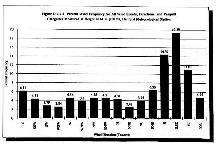
Two types of releases were modeled for this assessment. The first type is the ground release from the tank farms. Modeling for the ground release used the 9-year average (1983 to 1991) wind data measured at a height of 10 m (33 ft) above the Hanford Meteorological Station in the 200 Areas. Table D.2.2.1 displays the meteorological data (i.e., joint frequency distribution of wind speed, wind direction, and stability category) for all stability categories (Pasquill A-G). Figure D.2.2.1 illustrates the data in Table D.2.2.1 and shows a summary of wind direction frequencies. The second release type is the elevated release, which is a release emitted from a processing plant stack. Modeling for the elevated release used the 9-year average (1983 to 1991) wind data measured at a height of 61 m (200 ft) above the Hanford Meteorological Station for stacks taller than 10 m (33 ft). Table D.2.2.2 displays the meteorological data for all stability categories (Pasquill A-G). Figure D.2.2.2 illustrates the data in Table D.2.2.2 and provides a summary of wind direction frequencies.
Table D.2.2.2 Joint Frequency Data Collected at 61 m (200 ft) (1983 to 1991)
General Public
For the general public, the atmospheric transport and dispersion modeling was the same as applied for the noninvolved workers, but the distance from the release was changed to extend from the Site boundary to a distance of 80 km (50 mi).
Air Dispersion Isopleths
As discussed earlier, the air dispersion modeling for routine remediation was performed for two release categories: ground and elevated releases. Contour plots showing Chi/Q isopleths for these two cases are presented in Figures D.2.2.3 and D.2.2.4. These plots can be used to calculate the dose and risk to receptors at locations other than the maximally-exposed individual (MEI) locations presented in this assessment. The Chi/Q values shown were computed by GXQ Version 4 (Hey 1993 and 1994). Although the Chi/Q values used in the assessment were computed by GENII, GXQ was used for purposes of generating the contour plots because it requires less processor time than GENII. The computational methods used by GXQ are identical to those used by GENII.
Figure D.2.2.3 Chi/Q Isopleths for Ground Releases s/m3
Figure D.2.2.4 Chi/Q Isopleths for Elevated Releases in s/m3
D.2.2.3 Exposure
Exposure to the receptors for this analysis is from airborne contaminants and/or from direct exposure from gamma radiation fields. The radiological dose to a receptor would depend on the location of the receptor relative to the point of release of the radioactive material, or the shielding and distance of the receptor from the radiation field. Doses for the MEI and population were computed for each receptor class. The MEI worker is an individual that receives the highest annual exposure. The receptors are identified as follows.
- Worker population and MEI worker - These are individuals directly involved in the proposed remedial activities. They would receive exposure from inhalation and from direct exposure to gamma radiation fields during routine operation of TWRS facilities.
- Noninvolved worker population and MEI noninvolved worker - This was based on the current Hanford Site employment and assumed to be located from 100 m (330 ft) out to the Hanford Site boundary. Exposure would be by the inhalation pathway and by direct exposure from submersion in a radioactive cloud from routine air emissions during operation of TWRS facilities. The noninvolved worker population would receive a dose based on an annual average. The MEI noninvolved worker would receive the highest annual exposure.
- General public population and MEI general public - The general public
population includes people located within 80-km (50-mi) of the Hanford Site
boundary. They would be exposed through air dispersion of the plume, which
could result in inhalation, external exposure, and exposure from ingestion of
contaminated meat, dairy products, and vegetables. The MEI general public is
assumed to be an individual located at the Hanford Site boundary who receives
the highest annual exposure. The Site boundary is considered to be an adjusted
Hanford Site boundary that excludes areas likely to be released by DOE in the
near future. The Site boundary for the EIS was defined as follows:
- N. Columbia River - 0.4 km (0.25 mi) south of the south river bank;
- E. Columbia River - 0.4 km (0.25 mi) west of the west river bank;
- S. A line running west from the Columbia River, just north of the Washington Public Power Supply System leased area, through the Wye Barricade to State Route 240; and
- W. State Route 240 and State Route 24.
Potential exposure and subsequent carcinogenic risk and noncarcinogenic health hazards from chemical emissions were evaluated for the MEI worker, MEI noninvolved worker, and MEI general public receptors as described in more detail in the following text.
Radionuclide exposure estimates for the TWRS workers did not require using a computer model because fixed dose values were assumed to be similar to the values previously measured for similar activities at the Hanford Site. For exposure to nonradioactive chemical emissions, the MEI worker was evaluated using a "box" model. This model assumed that the MEI worker was located within a box 100 m long, 100 m wide, and 3 m high (330 ft long, 330 ft wide, and 10 ft high). Average wind velocity perpendicular to the side of the box was assumed to be 3.6 m/sec. Then, the Chi/Q (atmospheric dispersion coefficient) for the MEI worker was estimated using GENII as follows.
Chi/Q = 1 / (L) (H) (W)
Where:
Chi/Q = Sec/m3
L = Downwind length of the box, m
H = Height of the box, m
W = Average wind velocity, m/sec
The estimated Chi/Q value for the MEI worker was 9.26E-04 sec/m3.
For the noninvolved worker and general public, exposure was estimated through the use of the computer GENII model (Napier et al. 1988 and DOE 1995c). GENII was used to calculate doses corresponding to the Chi/Q values generated through air transport modeling. The GENII calculations were performed assuming that source term release and receptor intake end after 1 year (i.e., 8,760 hours). Doses calculated by GENII were multiplied by the duration (in years) of a particular activity to produce the total dose for that activity. The dose calculation ends after 70 years (i.e., a 70-year life expectancy is assumed).
The GENII computer program allows calculation of radiation doses to individuals or the population from airborne and waterborne radionuclide releases of radionuclides to the environment. Exposure pathways (i.e., ingestion, inhalation, and external exposure routes) are included. For the present analysis, exposure pathways are included in the dose analysis for inhalation or airborne activity, external exposure to airborne and deposited activity, and ingestion of agricultural products grown in soil contaminated from atmospheric deposition. Parameter values used in the analysis were as defined by Schreckhise et al. (Schreckhise et al. 1993) for dose analyses performed for Hanford Site activities. The parameters used for the individual and population dose analyses generally are more conservative than those used for the baseline and post-remediation analyses. The dose estimates generated by GENII were converted to risk as described in Section D.2.2.4.
The assumptions for estimating exposures to the receptors listed previously are described in the following sections.
Workers
The worker exposure is a combination of exposure from inhalation and direct radiation and would depend on the activity. The historical average dose for a Hanford Site tank farm worker has been 14 millirems per year (mrem/year) (WHC 1995g and Jacobs 1996). This same average is assumed for radiation workers during construction of the transfer lines, retrieval system tie-ins, and the tank farm confinement facilities. This same dose of 14 mrem/year is also assumed for monitoring, maintenance, and closure activities. A dose of 200 mrem/year is assumed for personnel operating the evaporators, retrieval facilities, separation and treatment facilities (both in situ and ex situ), and for processing the capsules. This was based on a dose of 200 mrem/year, average whole body deep exposure to operational personnel, at the Plutonium-Uranium Extraction (PUREX) Plant during 1986 (WHC 1995g and Jacobs 1996). A dose of 200 mrem/year was assumed for capsule alternatives. The MEI dose (one worker that receives the maximum exposure permissible) was based on a current site administrative control level of 500 mrem/year per worker for each year of operation.
For nonradiological chemicals, the chemical intake (dose) was estimated for the MEI worker according to the following equation:
| Intakei = (Cai) (IR) (EF) (ED) |
| (BW) (AT) |
Where:
Intakei = Inhalation intake of the ith chemical, mg/kg-day
Cai = Estimated air concentration of the ith chemical, mg/m3
IR = Worker inhalation rate, 20 m3/day
EF = Worker exposure frequency, 250 days/year
ED = Worker exposure duration, 30 years
BW = Worker body weight, 70 kg
AT = Averaging time, days
= (ED)(365 days/year) for noncarcinogens
= (70 years)(365 days/year) for carcinogens, (25,550 days)
Noninvolved Workers
During the workday, the noninvolved workers would be exposed to contamination from atmospheric emissions released during implementation of TWRS remedial activities. The noninvolved workers are assumed to occupy an area extending from 100 m (330 ft) out to the Hanford Site boundary. To calculate the noninvolved worker population dose, Hanford Site-specific population data were obtained from the Hanford Site phone directory and increased by 10 percent to account for uncertainties. The Hanford Site worker populations are presented in Table D.2.2.3.
Table D.2.2.3 Onsite Population
The principal assumption for calculations of dose is the breathing rate, which is assumed to be 3.30E-04 m 3 /sec (4.30E-04 yd 3 /sec). The dose from ingesting contaminated food was not included because it was assumed that ingestion of food grown onsite would not be allowed. The duration of exposure would vary depending on the schedule for each of the TWRS alternatives being considered.
The noninvolved MEI worker was assumed to be exposed from inhalation and external radiation from the plume continuously throughout the year and from deposited activity for half of the year (4,380 hr/yr). Chemical intake (dose) was estimated for the MEI noninvolved worker according to the same equation and exposure parameters used for the MEI workers. The noninvolved worker population was assumed to be exposed from inhalation and external radiation from the plume continuously throughout the year and from deposited activity for one-third of the year (2,920 hr/yr). The dose from inhalation of resuspended activity was evaluated using the mass loading approach with a particulate air concentration of 100 mg/m3 for both the maximum individual and population analyses.
General Public
The exposure pathways for the general public are inhalation, external exposure from submersion in a cloud, and consumption of fruits, vegetables, meat, and milk. The general public is assumed to occupy an area extending from the Hanford Site boundary to 80 km (50 mi) from the release site. Population data obtained from the 1990 Census (Beck et al. 1991) are used to calculate exposure and dose for the average member of the general public. Table D.2.2.4 displays the general public population within 80 km (50 mi) of the Hanford Site.
Table D.2.2.4 Offsite Population
For radiological emissions, the assumptions for the general public (MEI and population) were the same as for the noninvolved workers, but also included ingestion of contaminated farm products. The general public MEI was assumed to ingest the following foods: leafy vegetables (82 g/day), root vegetables (600 g/day), fruit (900 g/day), grain (220 g/day), beef (220 g/day), poultry (50 g/day), milk (740 g/day), and eggs (82 g/day). The individuals in the general population each were assumed to ingest the following foods: leafy vegetables (41 g/day), root vegetables (383 g/day), fruit (175 g/day), grain (197 g/day), beef (192 g/day), poultry (23 g/day), milk (630 g/day), and eggs (55 g/day). The maximum individual exposure is based on intake assumptions that have been used historically at the Hanford Site for risk analysis intended to show protection to the public.
For nonradiological chemicals, the chemical intake (dose) was estimated for the MEI general public receptor using a lifetime average daily dose (LADD). The LADD was the combined intake over 6 years for a child and over 24 years for an adult, resulting in a residential exposure duration of 30 years. The residential or general public intake was calculated according to the following equation:
| Intakei = (Cai) (IR) (EF) (ED) |
| (BW) (AT) |
Where:
Intakei = Inhalation intake of the ith chemical, mg/kg-day
Cai = Estimated air concentration of the ith chemical, mg/m3
IR = Residential inhalation rate, m3/day
= 20 m3/day for an adult
= 10 m3/day for a child
EF = Residential exposure frequency, 365 days/year
ED = Residential exposure duration, years
= 24 years for an adult
= 6 years for a child
BW = Residential body weight, kg
= 70 kg for an adult
= 16 kg for a child
AT = Averaging time, days
= (ED)(365 days/year) for noncarcinogens
= (70 years)(365 days/year) for carcinogens, (25,550 days)
Noncarcinogenic health effects were evaluated for a child intake because this scenario results in a larger exposure per body weight and would be more health protective for potential sensitive members of the general population. Carcinogenic effects were evaluated using the combined LADD. Potential impacts from deposition of suspended particulate and subsequent uptake from home-grown food products are based on the magnitude of the emissions and inhalation risks/hazards for residential receptors.
D.2.2.4 Risk
Routine risk for radionuclides is expressed in terms of latent cancer fatalities (LCFs). To estimate the number of cancer deaths that would result from exposure to low dose rates of ionizing radiation, dose-to-risk conversion factors are used to convert the calculated dose (from GENII) to a value for risk. Specific conversion factors were used that are accepted by agencies responsible for protection of human health and the environment, such as the Nuclear Regulatory Commission (NRC) (NRC 1991) and (EPA 1993a).
For radiological risk, two different conversion factors were used: one for workers and noninvolved workers and another for the general public, as recommended by the DOE Office of National Environmental Policy Act (NEPA) Oversight (DOE 1993d). The accepted dose-to-risk conversion factor for the worker is 4.0E-04 LCFs per person-rem effective dose equivalent (400 cancer deaths per million person-rem). The accepted conversion factor for the public is 5.0E-04 LCFs per person-rem effective dose equivalent (500 cancer deaths per million person-rem) (NRC 1991, ICRP 1991). The value for the public is higher because the public includes children, and children are more sensitive to radiation exposure. Assumptions for risk calculations are described in the following text.
In order to estimate the potential noncarcinogenic effects from exposure to multiple chemicals, the HI approach was used. The HI is defined as the summation of the hazard quotients (calculated dose divided by the reference dose [RfD]) for each chemical, for each route of exposure, and is represented by the following equation:
| HI | = | Calculated Dosea | + | Calculated Doseb | + | ... | + | Calculated Dosei |
| RfDa | RfDb | RfDi |
A total HI less than or equal to 1.0 (unity) is indicative of acceptable levels of exposure. To be truly additive in effect, chemicals must affect the same target organ system or result in the same critical toxic endpoint. Therefore, the approach listed previously is conservative and health protective in assuming that all chemical emissions are additive, and the approach provides a screening-level evaluation to potential noncarcinogenic effects.
Quantitative estimates of upper-bound incremental cancer risk (i.e., the excess cancer risk from fatal and nonfatal cancers) due to site-related chemicals were evaluated according to the following equation:
Ri = (qi) (Ei)
Where:
Ri = Estimated incremental risk of cancer associated with the chemical;
qi = Cancer slope factor for the chemical, (mg/kg-day)-1
Ei = Exposure dose for the chemical, mg/kg-day
Carcinogenic risk was assumed to be additive and was estimated by summing the upper-bound incremental cancer risk for all carcinogenic chemical emissions.
Workers
Worker risk was evaluated in terms of a maximum individual and collective radiation dose to the workforce. The worker risk was calculated both for each unit process and for each alternative or subalternative as a whole. The method of calculation was as follows:
R = (DR) (W) (risk factor of 4.0E-04 cancer fatality/person-rem) (1.0E-03 rem/mrem)
Where:
R = the number of incremental LCFs due to routine exposure
DR = is the exposure value previously discussed (i.e., 500 mrem/year for the MEI, 200 mrem/year per person, and 14 mrem/year per person)
W = the number of remediation workers exposed during processing for each alternative
For the MEI worker, the exposure assumed for the purposes of the EIS results in an annual risk of 2.0E-04 LCF (0.5 rem/year 4.0E-04 LCF/rem). The risk for an entire alternative would be the product of this annual risk and the alternative's duration in years. For the worker population exposure, the exposure and resulting risk would vary by alternative and are presented in Section D.4.0.
Noninvolved Workers
Risk was calculated for the MEI noninvolved worker and total population of noninvolved workers. The MEI noninvolved worker is located where the dose and risk are highest. This location would change as release conditions change. The dose and risk were calculated for the Site's total noninvolved worker population of approximately 10,900.
General Public
The MEI member of the general public is located where the dose and risk are highest. This location would change as release locations change with the various alternatives. The population dose and risk to the general public would be the total dose and risk to the general population of approximately 376,000 within an 80-km (50-mi) radius from the release point.
Transportation risk for routine remediation is the integrated risk from direct radiation exposure from onsite truck or rail transport of waste to and from TWRS processing facilities only. Offsite rail transport of waste to the proposed national high-level waste (HLW) repository is discussed in Volume Four, Section E.16.0.
Transportation risk has been estimated by Green (Green 1995) using the RADTRAN 4 computer code (Neuhauser and Kanipe 1986). A key variable in the code is the dose rate from the vehicle package. The radioactive shipments in this analysis were assumed to be the regulatory maximum dose rate of about 10 mrem per hour at 1 m (3.3 ft). It is likely that many of the shipments would have lower values.
For the onsite shipments, the average population density of the 200 East Area (DOE 1994) was assumed to be 264.4 persons/km2 (684.7 person/mi2). All onsite travel was assumed to be in a zone with this population density.
The population dose was multiplied by a dose-to-risk conversion factor to estimate the LCF. The worker conversion factor used was 4.0E-04 (400 cancer deaths per million person-rem effective dose equivalent). For the public, the conversion factor was 5.0E-04 (500 cancer deaths per million person-rem effective dose equivalent).
|
NEWSLETTER
|
| Join the GlobalSecurity.org mailing list |
|
|
|